Quantitative Value with Momentum

“Fundamentals tell you what to buy, technicals tell you when to buy it.”

1. The Quantitative Value with Momentum Philosophy

Value

Benjamin Graham, who made widely known the idea of purchasing stocks at a discount to their “intrinsic value” back in the 1930’s, is known today as the father of value investing. Since Graham’s time, academic research has shown that stocks trading at low price relative to their fundamentals (e.g. earnings, cash flows etc.) have historically outperformed the market [i]. In the investing world, Graham’s most famous student, Warren Buffett, has inspired legions of investors to adopt the value philosophy.

Momentum

Momentum investing is simply buying those stocks that have appreciated most relative to other stocks in a given universe. Moreover, when it comes to the “momentum” (formerly called “relative strength price momentum”) value investors tend to scoff at the idea that only the price of a stock could be used as a basis for investment. However, while we consider ourselves diehard value investors, we also consider ourselves evidence-based investors first and foremost.

Eugene Fama, the 2014 co-recipient of the Nobel Prize in Economics and father of the efficient market hypothesis, and his equally well-credentialed co-author, Ken French, have summarized the academic research on momentum as follows [ii]:

“The premier anomaly is momentum.”

When the greatest empirical finance researchers suggest momentum is the leading academic anomaly, we take note. Fama and French make this statement because the empirical research on the momentum effect is compelling. For example, academic researchers have examined stock data going back over 200 years and identified a significant and robust historical performance record [iii]. Momentum is well grounded, historically [iv]. Of course, for a strategy to provide persistent above average returns we need it to be steeped in a behavioural bias, and not simply possess a compelling backtest. We believe, the above average returns to momentum will persist because they are driven by innate human bias [v].

Value with Momentum

We know value investing works; we know momentum investing works; so, what is “value with momentum” and why do we combine two strategies that are known to work independently?

Here we turn to the wisdom of Warren Buffet, “Know your circle of competence, and stick within it. The size of that circle is not very important; knowing its boundaries, however, is vital.”

On deeper reflection, in our view, the “circle of competence” consists of two independent circles, technical and psychological. Where these circles intersect is where you are within both your technical and psychological circle of competence - “Total Competence” - you want to be there. Please refer to the diagram below for a graphical representation of this concept:

As evidence-based investors we are well versed in the ways of both value and momentum. However, momentum, while backed with centuries of evidence does not possess any underlying business fundamentals (e.g. sales, cash flows etc.) supporting its case, unlike value. This fact left us wondering for just how many years could we endure underperformance from a momentum strategy [vi] without wilting. After all, the best investing strategy is the one you can stick with! Our self-reflection resulted in the research and development of a strategy that is “founded on fundamentals and guided by technicals” - Quantitative Value with Momentum.

Human Behaviour & Quantitative Tools

Despite widespread knowledge that value and momentum generate higher returns over the long-haul, both strategies have continued to beat the market. How is this possible? The answer relates to a fundamental truth: human beings behave irrationally. We follow an evolutionary mindset that focuses on survival, not return optimization. While we are unlikely to ever eliminate our survival instincts, we can minimize their impact by employing quantitative tools.

“Quantitative,” is often considered to be an opaque mathematical black art, only practiced by Ivory Tower academics and supercomputers. However, quantitative (or systematic) processes are merely tools that value investors can use to minimize their “survival” instincts when investing. Quantitative tools serve two purposes: 1) protect us from our own behavioural errors, and 2) exploit the behavioural errors of others. These tools do not need to be complex, but they do need to be systematic. The research demonstrates that simple, systematic processes outperform human “experts” [vii]. The inability of human beings to robustly outperform simple systematic processes also holds true for investing, just as it holds true for most other fields [viii].

Much of the analysis conducted by investors - reading financial statements, interpreting past trends, and assessing relative valuations - can be done faster, more effectively, and across a wider swath of securities via a systematic process. Investors argue that instinct and experience add value in the stock-selection process, but the evidence does not support this interpretation. Why? When investors respond to non-quantitative signals (e.g., the latest headlines, their expert friend’s opinion, their interpretation of a price pattern etc.), they unconsciously introduce cognitive biases into their investment process. These biases lead to predictable underperformance. The Quantitative Value with Momentum Investing Philosophy is best suited for value investors who can acknowledge their own fallibility. Granted, the approach is not infallible, and should always be questioned; however, the approach seeks to provide the following: a systematic, evidence-based, value/momentum focused investment strategy that is built to beat behavioural bias [ix].

2. The Quantitative Value with Momentum Process

We distilled our entire process into six core steps:

Step 1 - Identify Universe

We consider the global stock universe with a focus on developed markets, but candidates in some emerging markets are also considered. However, as financial institutions (e.g. banks) report their accounting information differently to firms in other industries we exclude them from our portfolio.

Step 2 - Forensic Accounting Screens

As notable value investor Seth Klarman has advised, “Loss avoidance must be the cornerstone of your investment philosophy.” Therefore, we seek to eliminate those firms that risk causing a permanent loss of capital.

To identify those firms that represent the greatest threat to our capital we apply empirically proven quantitative tools.

Accrual Red Flags

Earnings represent an accounting measure of a firm’s profitability (or loss) and are constructed using the accruals method of accounting. Simply put, the often-vaunted earnings figure sitting at the foot of an income statement does not represent cash, and it is susceptible to manipulation. So, to identify those firms that possess an extreme level of accruals we utilise a simplified version of the Scaled Total Accruals (STA) [x] model researched in the paper “Do Stock Prices Fully Reflect Information in Accruals and Cash Flows about Future Earnings?” [xi]

STA = (Net Income – Cash Flow from Operations) / Total Assets

In addition, we utilise the Scaled Net Operating Assets (SNOA) model examined in the paper “Do Investors Overvalue Firms With Bloated Balance Sheets?” [xii] The authors observe that when the growth in cumulative accruals (net operating income) outstrips the growth in cumulative free cash flow, the balance sheet becomes “bloated,” and firms find it increasingly difficult to sustain earnings growth. During the 1964 to 2002 sample period, the authors find that net operating assets scaled by total assets is a strong predictor of poor long-term stock returns [xiii].

SNOA = (Operating Assets – Operating Liabilities) / Total Assets

Earnings Manipulation

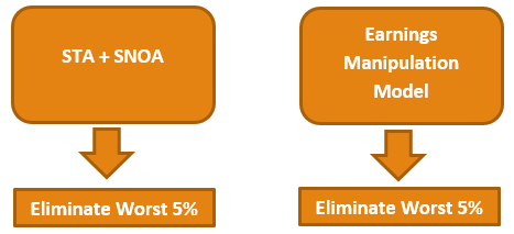
We have replicated the “Earnings Manipulation Model” developed by Professor Beneish as detailed in his research paper “The Predictable Cost of Earnings Manipulation” [xiv]. While statistically sophisticated and highly technical in nature the principles of the model are intuitive and deal with changes in: receivables, gross margins, asset quality, sales growth, depreciation, expenses, leverage, assets and accruals. Collectively the model scales the output score from each of the variables and identifies those firms that are at a greater probability of manipulating their earnings - we avoid them!

The graphic below depicts the Capital Preservation Screening process:

Step 3 - Valuation Screen

A plethora of research and writing exists with regard to valuation metrics and their utility. To ensure the highest level of efficacy in the construction of our valuation screen we concentrated our research efforts on the books and research papers published by well renowned quantitative investment managers and academics which included: “What Works on Wall Street (Forth Edition)” by Jim O’Shaughnessy, “Quantitative Value” by Wesley Gray and Tobias Carlisle, “Global Value” by Mebane Faber, “Shareholder Yield” by Mebane Faber, “Analyzing Valuation Measures: A Performance Horse-Race over the past 40 Years” by Wesley Gray and Jack Vogel.

We reviewed the evidence which measured the returns achieved by no less than 11 single factor valuation metrics including:

Price to Book;
Price to Earnings;
Earnings before Interest, Taxes and Depreciation and Amortization (EBITDA) to Enterprise Value (EV);
Price to Cash Flow;
Price to Sales;
Dividend Yield;
Buyback Yield;
Return on Equity;
Earnings before Interest and Taxes (EBIT) to EV;
Free Cash Flow (FCF) to EV; and
Gross Profit to EV.

We then considered the wisdom of using a multiyear metric as implied by none other than Benjamin Graham in “Security Analysis” so as to avoid pitfalls of the business cycle. While it was found that some merit may exist in using multiyear metrics the evidence was mixed and that the additional predictive capability of multiyear metrics was marginal.

Finally, the virtue of a composite valuation metric was also considered. In the case of composite value metrics, the back tests contained in “Quantitative Value” found that the simple, one-year EBIT/EV performed better than any composite valuation metric, including those that incorporated multiyear periods. It should be noted that their universe focussed on stocks above the 40th percentile on the New York Stock Exchange i.e. on December 31, 2011, the smallest stock in their investable universe had a market capitalization of $1.4 billion. In contrast the evidence uncovered in “What Works in Wall Street (Forth Edition)” found that the best performing valuation metric was indeed a composite. Here it should be noted that the back tests for “All Firms” did include firms with market capitalizations down to an inflation adjusted USD 200 million (in 2009 dollars) which would have influenced the results, in addition to the differences in the actual metrics used to construct the composite valuation metric.

Given we do not impose any market capitalization restrictions on our investment universe and taking into consideration that the fundamentals of smaller firms tend to be more volatile compared to those of larger firms we thought it prudent to adopt a composite value metric and thus ensure our investment candidates were “cheap” from a variety of angles.

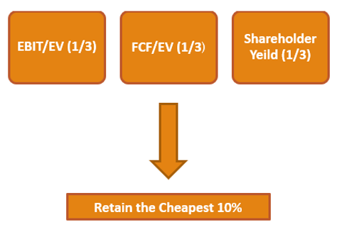
The next challenge we faced was to determine which metrics to use in our composite value screen. We settled on the following, each weighted at one third.

EBIT to EV;
FCF to EV; and
Shareholder Yield (itself composed of: 1/3 Buyback Yield; 1/3 Debt Paydown Yield, 1/3 Dividend Yield).

For reference EBIT to EV was the best performing valuation metric examined in the book “Quantitative Value” over the period from 1964 to 2011. FCF to EV was the second-best valuation metric identified in research paper “Analyzing Valuation Measures: A Performance Horse-Race over the past 40 Years” over the period from 1971 to 2010 [xv]. Lastly, Shareholder Yield was analysed extensively in the book “Shareholder Yield” by Mebane Faber where it was shown to materially outperform the S&P 500 from 1982 to 2011.

The graphic below depicts the Valuation Screening process:

Step 4 - Generic Momentum Screen

To a value investor buying a stock because it has gone up in price sounds like an idea that runs the continuum from a masochistic desire to destroy capital to outright lunacy! The ever-mounting body of evidence, however, suggests that such a strategy belongs in the domain of the rational empiricist.

Momentum can be calculated in numerous ways; while some periods of measurement are additive to returns, others are outright destructive and need to be avoided.

Academic research for three different look-back periods is summarized below:

Short-Term Momentum (1-month) - exhibits a reversal in returns [xvi]
Long-Term Momentum (3 to 5 years) - exhibits a reversal in returns [xvii]
Intermediate-Term Momentum (6-12 months) - exhibits a continuation in returns [xviii]

In short, both short-term and long-term momentum signal a future reversal in returns. In other words, one can expect these stocks to underperform. However, intermediate-term momentum provides a continuation of returns - these stocks tend to outperform and are the subject of our focus.

The momentum look-back we use as part of our generic momentum screen is calculated using the cumulative 12-month past returns, excluding the most recent month (“12_2 momentum”). We exclude the most recent month as 1-month periods exhibit a reversal in returns; therefore, excluding the most recent month minimizes the effect of short-term momentum reversal. Strictly speaking, we calculate momentum using the cumulative returns over 11 months.

Wesley Gray and Jack Vogel in their book, “Quantitative Momentum” [xix] examine how the momentum portfolios have performed. Specifically, they analyse the returns to the value-weighted top and bottom decile momentum portfolios using 12_2 momentum from 1-Jan-1927 to 31-Dec-2014 rebalanced monthly.

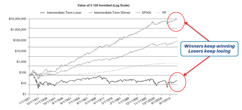
Clearly from their analysis we can see that buying the highest momentum stocks (and rebalancing monthly) over the time period tested worked remarkably well.

To illustrate the importance of rebalancing momentum we provide an extract from the research piece “How Portfolio Construction Affects Momentum Funds” [xx]:

Clearly, there is a relationship between the holding period (the number of firms) and returns. The holding period is important; keeping the number of firms constant, the lower the holding period, the higher the CAGR. Such is the decay in momentum that a 12-month holding period resulted in return below that of the overall universe for a 50-stock portfolio. However, due to the impact of commissions (assuming 0.1% per trade) a 3-month rebalance represents the optimal rebalancing period; therefore, this is the period we implement in our process.

At this point in the process we retain the 10% of stocks with the highest momentum:

Step 5 - Momentum Quality Ranking

“All momentum is not created equal”

Having identified our universe, removed those stocks that presented us with the greatest risk of permanently destroying capital, identified the cheapest decile of stocks using our composite value metric and determined which of those stocks demonstrate the greatest generic (i.e. 12_2) momentum we now rank our remaining candidates based on the “quality” of their momentum.

But what is “quality” momentum and how does it differ from the “generic” momentum we identified in the previous step?

Jack Vogel of Alpha Architect explains quality momentum as follows:

The details for calculating momentum quality are complex, but the intuition is simple. Consider two hypothetical momentum stocks: Stock A is a box store, Stock B is a biotechnology company, and both companies have a 200% return over the past 12 months. However, assume A and B have vastly different paths to 200% returns.

Buzzing Biotech: Stock B’s returns were 0% for 11 months, but just recently Stock B was granted an FDA approval for a new drug and the stock shot up 200%.
Boring BigBox Store: Stock A has returned 0.80% each day, on average, for the past 250 days, and has generated a 200% return.

Stock A and Stock B are both considered momentum stocks, but Buzzing Biotech’s path is much different from Boring BigBox’s path. So-called “path dependency” matters, if momentum is driven by an investor bias referred to as “limited attention.” For example, Buzzing Biotech’s FDA approval will likely be covered by the media and be highly available to investors, thus rapidly driving the company’s price to efficient levels. However, Boring BigBox is delivering news that is consistently better than market expectations over a longer period, and because the attention to Boring BigBox is limited, this good news is slow to be incorporated into market prices. Below we graphically depict a hypothetical example of 2 “high” momentum stocks.

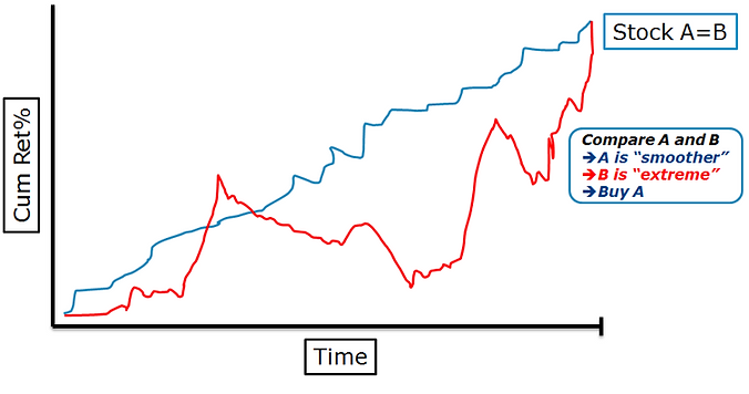
Although testing the “limited attention” hypothesis in the context of momentum is challenging, we’re lucky that finance professors have been hard at work. In a 2014 paper titled, “Frog-in-the-Pan: Continuous Information and Momentum,” Zhi Da, Umit Gurun, and Mith Awarachka find that high momentum firms with smooth, or “high-quality” momentum, tend to do better than those firms with choppy low-quality momentum [xxi].

In this step of the process we rank the remaining stocks on the quality of their momentum:

Step 6 - Construct & Manage

Steps 1 to 5 systematically seek to identify the lowest risk, cheapest, highest quality momentum stocks. However, we still need to specify how we construct and manage the portfolio.

The components of portfolio construction and management are addressed below:

Defining “Risk” - we define risk as the probability of the permanent loss of capital rather than volatility or any variant thereof. The permanent loss of capital when investing in equities is possible. While it is said that finance suffers from “physics envy”, we think an adaption of the law of conservation of energy applies to investing; “risk cannot be destroyed, only changed from one form to another”.

Currency Risk - constructing a global equity portfolio creates exposure to foreign currencies (we usually convert the base currency into the local currency when investing in stocks denominated in a non-base currency), and we do not hedge against it. This is primarily because we do not necessarily see foreign currency fluctuations as a risk; on the contrary, we see hedging foreign currency exposure as creating a “concentration risk” in a single currency. However, we might consider hedging currency exposure if, for example, a currency stretched far from its 5-year average relative to other currencies, or some other extraordinary situation presented itself.

Weighting - we equally weight our holdings. In a 2009 study by DeMiguel, Garlappi, and Uppal, “Optimal Versus Naïve Diversification,” the authors found that a basic equal-weight asset allocation model beats modern portfolio theory and 13 other even more complex strategies [xxii]. We heed the lesson that “simplicity trumps complexity” and consequently we simply aim to “equal weight” our holdings.

Number of holdings - we generally hold 20 to 25 stocks in equal weight (at cost). We accept that investing in stocks can result in the permanent loss of capital. Accordingly, one divided the number of holdings reflects that proportion of capital we accept could be lost in any given stock. From an academic perspective, Elton and Gruber’s 1977 paper, “Risk Reduction and Portfolio Size: An Analytical Solution” draws the conclusion that the bulk of “diversification benefit” is achieved with just 8 stocks and becomes negligible beyond 50 stocks [xxiii]. In addition, table 4.2 in the book “Concentrated Investing: Strategies of the World's Greatest Concentrated Value Investors” [xxiv], by Allen C. Benello, Michael van Biema, and Tobias E. Carlisle it is demonstrated that over time a relatively small sample, when picked at random can replicate the returns of a much larger population; the conclusion being one need not own “too many” stocks to achieve the “benefit of diversification”.

Rebalancing - following entry into the portfolio, stocks are held for a minimum of 3 months. In the event that a stock remains in the portfolio after an initial 3 month hold it is reassessed on a monthly basis thereafter. Furthermore, in an attempt to reduce “whipsaws” (i.e., stocks bouncing in and out of the portfolio resulting in unnecessary turnover) the “value” and “momentum” parameters for retaining a stock are marginally extended. As addressed in an earlier section it is well known the momentum works best when rebalanced monthly. Nonetheless, due to the impact of commissions a 3-month rebalance represents the optimal rebalancing period; therefore, this is the period we implement in our process. However, rebalancing warrants further discussion - while 3-months represents the optimal (after commissions) rebalancing period for a “pure momentum” strategy, is it the best rebalancing period for a strategy that is essentially a value strategy with a momentum overlay? In an extensive research piece, “How to Combine Value and Momentum Investing Strategies” [xxv], it was established that more frequent rebalancing of such a strategy is preferable. Interestingly, even rebalancing a pure value strategy on a monthly basis (gross of fees) has been shown to be performance enhancing per the evidence contained in the research paper “On the Performance of Cyclically Adjusted Valuation Measures” [xxvi].

Final checks – in addition to that outlined above, prior to making the decision to invest, or otherwise, we analyse several items, including, but not limited to: insider transactions, short interest, audit reports, recent announcements etc. in an attempt to ensure the probability of incurring a permanent loss of capital is further reduced.

The complete Quantitative Value with Momentum algorithm is as follows:

3. Performance

Having outlined the process in detail we will now examine the historical returns.

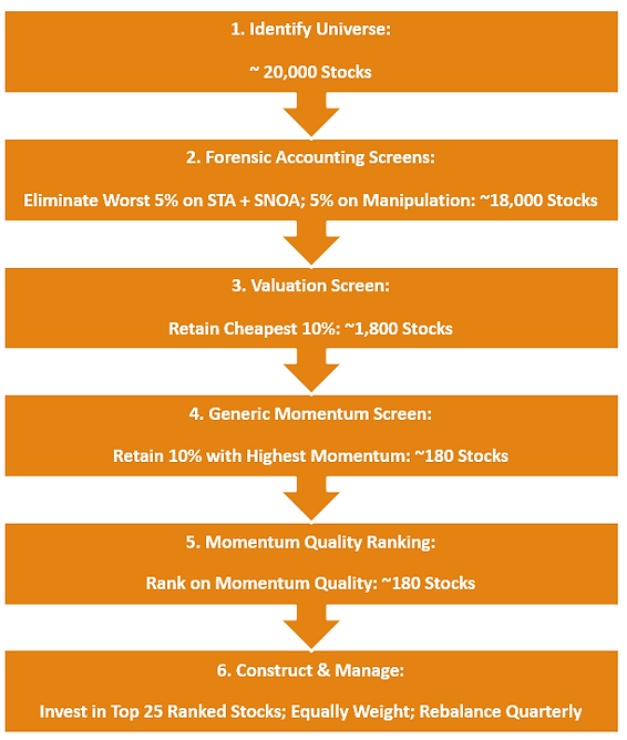
While no historical back-test of our exact process has been conducted, the “Trending Value” strategy examined in Chapter 27 of “What Works on Wall Street (Forth Edition)” by Jim O’Shaughnessy is somewhat comparable. The Trending value portfolio identifies the cheapest decile of stocks using a composite value metric and then sorts them by 6-month price appreciation (i.e. momentum). We specify the parameters and performance of the Trending Value strategy below:

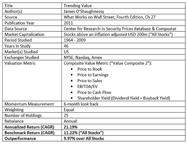
Not only did the Trending Value portfolio nearly double the benchmark, it never had a 5-year period where it lost money and it beat its corresponding universe, “All Stocks” in 100% of rolling 5-year periods and 99% of rolling 3-year periods!

Combining value and momentum is a winning strategy!

It should be noted that while this strategy combines value and momentum, the construction (i.e. sorting on the cheapest decile of value first, then sorting on momentum) renders it a value strategy first and foremost. To illustrate its association with “value” we note that the Trending Value portfolio returned 7.41% during the mania of dot.com bubble in 1999 whereas stocks sorted purely on 6-month price appreciation (i.e. disregarding value) generated returns of 100.64%.

Furthermore, it should be noted that investing in only the cheapest decile as identified by the composite valuation metric (“Value Composite 2”) a compound annual growth rate of 17.30% was achieved [xxvii]. For reference, the average number of stocks examined in any given year was 3,549 [xxviii]. Therefore, the average number of stocks in a decile was approximately 355. Furthermore, we can only assume that investing in the cheapest 25 stocks (as opposed to the cheapest decile), as identified by Value Composite 2 would have generated even higher returns.

While we do not have the tools at our disposal to decompose the returns of Trending Value into its various factors (e.g. market beta, value, size, momentum) through regression analysis, a rudimentary analysis provides an indication as to the potential drivers of return. Specifically, we know the “All Stocks” universe returned 11.22% and that Value Composite 2 returned 17.30% and Trending Value returned 21.19%. That is to say, adding Value Composite 2 increased returns by 54.19% [1] and adding momentum added an additional 22.49% [2] to returns. Analyzed another way, and roughly speaking, “value” contributed 60.98% [3] of the excess return and “momentum” added 39.02% [4] of the excess return.

Having specified the returns, portfolio construction and management of a somewhat comparable strategy, Trending Value, we will now turn our attention back to the Quantitative Value with Momentum process, identifying where and how our system is similar or where we have applied academic and practitioner research to improve upon Trending Value:

Universe - our investment universe has no restrictions on the market capitalization of stocks, and in addition we invest globally. This means not only do we have a far larger universe we also create the opportunity to capture the additional return associated with the “size factor” [xxix] [xxx] [xxxi] [xxxii].

Forensic Accounting Screens - our universe has been cleansed of those firms that are most likely to result in the permanent loss of capital thereby increasing returns (by reducing losers).

Valuation Screen - our respective composite value metrics are comparable.

Generic Momentum Screen & Momentum Quality - a large divergence exists when it comes to how we measure and implement momentum and this represents a significant area of improvement for Quantitative Value with Momentum over Trending Value. Not only do we use a look-back period that minimises the impact of short-term trend reversals we also implement a conceptually intuitive (but technically sophisticated) smoothed momentum screen to identify the stocks that possess the highest quality momentum.

Rebalancing - Trending Value was rebalanced annually [xxxiii] .However, as addressed in an earlier section it is well known the momentum works best when rebalanced monthly. Nonetheless, due to the impact of commissions 3-months represents the optimal rebalancing period; therefore, this is the period we implement in our process. The impact of more frequent rebalancing is significant and is a likely source of a material level of outperformance of Quantitative Value with Momentum vs Trending Value.

Given the material improvements we have made to key components of Trending Value in developing the Quantitative Value with Momentum process we are confident the returns would be significantly higher.

4. Conclusion - “Simple, but not easy”

“Investing is simple, but not easy” (Warren Buffett)

Investing in a strategy that combines value and momentum is theoretically “simple” but certainly not “easy”. Complexities in implementation aside, firms falling into the cheapest decile of a global stock universe are often ugly and facing problems. However, the empirical evidence is clear, in aggregate they greatly outperform the market over time. Moreover, even when enhancing their return profile by adding a momentum overlay to a portfolio of deeply undervalued stocks there are times when such a strategy may lag the market. Without a time horizon of at least 3 years an investor may not be “in the game” long enough to capture the rewards of the Quantitative Value with Momentum process; “no pain, no premium”.

In periods where people expect certain businesses to grow indefinitely or in speculative manias like the “dot com” bubble of the late 90’s, tried and tested strategies like value with momentum are likely to get left behind as capital gets drawn to a more compelling narrative. Moreover, notwithstanding their bargain basement price and momentum, when markets tumble firms identified by the Quantitative Value with Momentum process are unlikely to be spared.

The strategy requires an individual or fund to expend considerable resources to construct, maintain and manage such a system. Nonetheless, for the enterprising investor, with a sufficient time horizon, history tells us that the Quantitative Value with Momentum strategy will provide ample reward.

References

[1] (17.30% - 11.22%)/11.22% = 54.19%

[2] (21.19% - 17.30%)/17.30%) = 22.49%

[3] (21.19% - 11.22% = 9.97%; 17.30% - 11.22% = 6.08%; 6.08% / 9.97%) = 60.98%

[4] (21.19% - 11.22% = 9.97%; 21.19% - 17.30% = 3.89%; 3.89% / 9.97%) = 39.02%

[i] Wesley Gray and Jack Vogel, “Analyzing Valuation Measures: A Performance Horse-Race over the Past 40 Years.” 2012.

[ii] Fama, E. and K. French, 2008, Dissecting Anomalies, The Journal of Finance, 63, pg. 1653-1678.

[iii] Geczy, C. and M. Samonov, Two Centuries of Price Return Momentum, 2016. https://papers.ssrn.com/sol3/papers.cfm?abstract_id=2292544

[iv] The Quantitative Momentum Investing Philosophy, Jack Vogel, 2015. https://alphaarchitect.com/2015/12/01/quantitative-momentum-investing-philosophy/

[v] William N. Goetzmanny Simon Huangz, Momentum in Imperial Russia, 2018. https://papers.ssrn.com/sol3/papers.cfm?abstract_id=2663482

[vi] Is momentum investing dead? Or is it just painful?, Wesley Gray, 2016. https://alphaarchitect.com/2016/09/07/is-momentum-investing-dead-or-is-it-just-painful/

[vii] Painting by Numbers: An Ode to Quant, https://alphaarchitect.com/wp-content/uploads/2013/01/Painting-by-the-Numbers.pdf

[viii] Grove, W., Zald, D., Lebow, B., and B. Nelson, 2000, “Clinical Versus Mechanical Prediction: A Meta-Analysis,” Psychological Assessment 12, p. 19-30.

[ix] The Quantitative Momentum Investing Philosophy, Jack Vogel, 2015. https://alphaarchitect.com/2015/12/01/quantitative-momentum-investing-philosophy/

[x] Wesley Gray and Tobias Carlisle, Quantitative Value, Chapter 3 (New Jersey: John Wiley & Sons,2012).

[xi] Richard Sloan, “Do Stock Prices Fully Reflect Information in Accruals and Cash Flows about Future Earnings?” Accounting Review 71 (1996): 289–315.

[xii] David Hirshleifer, Kewei Hou, Siew Hong Teoh, and Yinglei Zhang, “Do Stock Prices Fully Reflect Information in Accruals and Cash Flows about Future Earnings?” Journal of Accounting and Economics 38 (2004): 297–331.

[xiii] Wesley Gray and Tobias Carlisle, Quantitative Value, Chapter 3 (New Jersey: John Wiley & Sons,2012).

[xiv] The Predictable Cost of Earnings Manipulation, Messod Daniel Beneish, Craig Nichols, 2007. https://papers.ssrn.com/sol3/papers.cfm?abstract_id=1006840

[xv] While Price to Book possesses the advantage of being focused on the balance sheet from where we can most easily obtain a statistical “margin of safety” its efficacy has been brought into question (refer Price-to-Book’s Growing Blind Spot, Chris Meredith, O’Shaughnessy Asset Management, LLC 2016). Following extensive review (and in light of other strategies we utilise) it was removed from the value composite after being included in the original version.

[xvi] Lehman, B. N., 1990, Fads, Martingales, and Market Efficiency, The Quarterly Journal of Economics, 105, pp. 1-28 and Jegadeesh, N., 1990, Evidence of Predictable Behavior of Security Returns, The Journal of Finance, 45, pp. 881-898.

[xvii] DeBondt, W. F., and R. Thaler, 1985, Does the Stock Market Overreact?, The Journal of Finance, 40, pp. 793-805.

[xviii] Jegadeesh, N., and S. Titman, 1993, Returns to Buying Winners and Selling Losers: Implications for Stock Market Efficiency, The Journal of Finance, 48, pp. 65-91.

[xix] Wesley Gray, Jack Vogel, Quantitative Momentum: A Practitioner's Guide to Building a Momentum-Based Stock Selection System (Wiley Finance), 2016.

[xx] How Portfolio Construction Affects Momentum Funds, Jack Vogel,2015. https://alphaarchitect.com/2015/11/16/how-portfolio-construction-affects-momentum-funds/

[xxi] Da, Z., U. G. Gurun, and M. Warachka, 2014, Frog in the Pan: Continuous Information and Momentum, Review of Financial Studies, pp. 1-48. https://www3.nd.edu/~zda/Frog.pdf

[xxii] V. DeMiguel, L. Garlappi, and R. Uppal, “Optimal Versus Naïve Diversification: How Inefficient is the 1/N Portfolio Strategy?” Review of Financial Studies 22, no. 5 (2009): 1915–1953.

[xxii] Elton, E. and Martin Gruber, 1977, Risk Reduction and Portfolio Size: An Analytical Solution, The Journal of Business 50, p 415-437.

[xxii] James O'Shaughnessy, What Works on Wall Street: The Classic Guide to the Best-Performing Investment Strategies of All Time, 4th ed. Chapter 4 Section 4 (New York: McGraw-Hill, 2011).

[xxiv] Allen C. Benello, Michael van Biema, and Tobias E. Carlisle, Concentrated Investing: Strategies of the World's Greatest Concentrated Value Investors”, 2016.

[xxv] How to Combine Value and Momentum Investing Strategies, Jack Vogel, 2015. https://alphaarchitect.com/2015/03/26/the-best-way-to-combine-value-and-momentum-investing-strategies/

[xxvi] Wesley Gray and Jack Vogel, “On the Performance of Cyclically Adjusted Valuation Measures” 2013. https://papers.ssrn.com/sol3/papers.cfm?abstract_id=2329948

[xxvii] James O'Shaughnessy, What Works on Wall Street: The Classic Guide to the Best-Performing Investment Strategies of All Time, 4th ed. Table 27.2 (New York: McGraw-Hill, 2011).

[xxviii] James O'Shaughnessy, What Works on Wall Street: The Classic Guide to the Best-Performing Investment Strategies of All Time, 4th ed. Table 4.2 (New York: McGraw-Hill, 2011).

[xxix] What Has Worked In Investing, Tweedy, Browne Company LLC, 2009, Table 5, pg 7. https://www.tweedy.com/resources/library_docs/papers/WhatHasWorkedFundOct14Web.pdf

[xxx] Asness, Frazzini, Israel, Moskowitz, Pedersen, “Size Matters, If You Control Your Junk”, 2015. https://papers.ssrn.com/sol3/papers.cfm?abstract_id=2553889

[xxxi] Does the Small-cap “size” effect exist? Probably, Wesley Gray, 2014. https://alphaarchitect.com/2014/07/02/does-the-small-cap-size-effect-exist-probably/

[xxxii] Chee Seng Cheong A Fin, Justin Steinert, “The size effect: Australian evidence”, Australasian Journal of Applied Finance, 2013.

Disclaimer

We are not registered investment advisors. This material has been provided for informational purposes only and should not be considered as investment advice or a recommendation of any particular security, strategy or investment product. Information contained herein has been obtained from sources believed to be reliable, but not guaranteed.